Neural networks are a powerful tool for teaching computers to recognize complex patterns, and now tools like Keras and TensorFlow are beginning to make them a practical tool for programmers who don't have a PhD in machine learning.

One very powerful aspect of these tools is the ability to share pre-trained models with others. There are many tutorials and courses that will walk you through the process of building a neural net and training it on some data set. But in other areas of software development we are far more likely to use off-the-shelf implementations of common algorithms rather than rolling them ourselves. We might work through implementing a sort algorithm or a binary tree in order to better understand the concepts, but having done so we almost always end up using the algorithms that come built in to our language or programming environment.

I suspect we'll see the same sort of thing happen in the machine learning world. While being able to train models on our own data will continue to be extremely valuable, there will be many cases where a model already exists that does what we want, and we'll just want to plug it in to our data.

Keras already provides some pre-trained models: in this article, I'll use the Inception V3 model to classify an image.

import numpy as np
import keras

from keras.preprocessing import image
from keras.applications.inception_v3 import decode_predictions
from keras.applications.inception_v3 import preprocess_input

Load the pre-trained model

inception=keras.applications.inception_v3.InceptionV3(
    include_top=True, 
    weights='imagenet', 
    input_tensor=None, 
    input_shape=None
)

(This actually downloads the weights from github. Keras saves your model files in ~/.keras/models in the HDF5 file format.)

!ls  ~/.keras/models

inception_v3_weights_tf_dim_ordering_tf_kernels.h5

inception

<keras.engine.training.Model at 0x7f6946e537b8>

inception.summary()

____________________________________________________________________________________________________
Layer (type)                     Output Shape          Param #     Connected to                     
====================================================================================================
input_1 (InputLayer)             (None, 299, 299, 3)   0                                            
____________________________________________________________________________________________________
conv2d_1 (Conv2D)                (None, 149, 149, 32)  864                                          
____________________________________________________________________________________________________
batch_normalization_1 (BatchNorm (None, 149, 149, 32)  96


(snipped several hundred lines here...)



mixed10 (Concatenate)            (None, 8, 8, 2048)    0                                            
____________________________________________________________________________________________________
avg_pool (GlobalAveragePooling2D (None, 2048)          0                                            
____________________________________________________________________________________________________
predictions (Dense)              (None, 1000)          2049000                                      
====================================================================================================
Total params: 23,851,784.0
Trainable params: 23,817,352.0
Non-trainable params: 34,432.0
____________________________________________________________________________________________________

Now let's load an image and see if Inception can recognize it

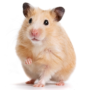
img = image.load_img('./hamster.jpg',target_size=(299,299))

img

Keras requires the input data to be in a specific shape.

x = image.img_to_array(img)
x = np.expand_dims(x, axis=0)
x = preprocess_input(x)

x.shape

(1, 299, 299, 3)

predictions = inception.predict(x)
prediction  = decode_predictions(predictions)[0][0]
prediction

('n02342885', 'hamster', 0.91639304)

And we're done

Inception is pretty confident that this is a picture of a hamster. Without having to do any training ourselves, or really having to know anything at all about neural networks, we've leveraged a publicly available model to classify our image.

Keras is a high-level neural network Python library, designed to sit on top of lower level implementations such as TensorFlow.

It provides abstractions that enable you to quickly create neural network structures. Here I'm going to try to create a simple 3 layer network, and use it to solve a basic classification problem.

For reference, the problem I'm trying to solve, and the network I'm using to solve it, are roughly equivalent to this interactive example at playground.tensorflow.org

Tell Jupyter to display matlplotlib plots directly in the notebook

%matplotlib inline

Imports

A lot of machine learning work ends up being about 'housekeeping' - finding, filtering, parsing, loading data, transforming it into a usable shape, and so on. The Pandas library is excellent for this type of work

import pandas as pd

Numpy is commonly used for creating and managing arrays of numbers and performing a wide variety of mathematical operations on them. Matplotlib and seaborn provide a number of useful plotting functions.

import numpy as np
import matplotlib.pyplot as pl

import seaborn
seaborn.set()

TensorFlow is Google's Machine Learning library

import tensorflow as tf

This is a useful function for splitting data sets into training and testing subsets.

from sklearn.model_selection import train_test_split

And finally Keras is the library I actually want to explore. My understanding is that it provides a high-level abstraction to common TensorFlow operations

import keras
from keras.layers import Dense, Activation

Create training data.

I'm going to create an array of data with two features, x1 and x2

data = pd.DataFrame(np.random.random((1500,2))*20 - 10,columns=['x1','x2'])

For simpler visualisation, I'm going to filter out values that lie very close to the axes.

data= data[(np.abs(data.x1)>1)& (np.abs(data.x2)>1)][0:1000]

And then for each (x1,x2) pair, I'm going to assign a value y that is true if x*y is greater than 0.

data['y']=((data.x1*data.x2)>0)

data.head()

Visualize the input data

Seaborn provides a function that gives me exactly the visualization that I want:

seaborn.lmplot(x="x1", y="x2", hue="y", data=data,fit_reg=False)

<seaborn.axisgrid.FacetGrid at 0x7efd8407dd68>

So we have two classes, and we're going to see if we can create a neural network that can distinguish between the two.

Create training data and test data

We assign 80% of the data to the training set, with the remaining 20% left over for testing the accuracy of our hypothesis.

train,test=train_test_split(data,train_size=0.8)

len(train), len(test)

(800, 200)

Keras seems to require input data in the form of Numpy arrays, so we extract those from our Pandas dataframe:

X_train = train[['x1','x2']].values
Y_train = train['y'].values

Define a neural network

Now we can use Keras to define our network. I'm going to specify a network with an input layer, an output layer, and a 4-node hidden layer.

model=keras.models.Sequential()

model.add(Dense(output_dim=4, input_dim=2,activation='tanh'))
model.add(Dense(output_dim=2,  activation='tanh'))
model.add(Dense(output_dim=1,  activation='tanh'))

Train the network

This is the bit that would take considerably more lines of code in a lower-level library. I can tweak parameters such as the cost function, the optimizer and so on. Here I choose a mean-squared-error cost function and a stochastic gradient descent optimizer.

I haven't yet figured out how to change the learning rate, which would be very helpful to know.

%%time
model.compile(loss='mean_squared_error', optimizer='sgd')

model.fit(X_train,
          Y_train,
          nb_epoch=250,
          batch_size=40,
          verbose=0)

CPU times: user 3.26 s, sys: 40 ms, total: 3.3 s
Wall time: 3.34 s

Having trained the network, check it against the test data.

plotPrediction runs the predict_classes method to attempt to classify the test data we provide, and then displays its guesses:

def plotPrediction(data,model):
    X = data.ix[:,:-1].values
    Y = data['y'].values

    d=data.copy()
    d['pred']=model.predict_classes(X,verbose=0).reshape(len(X))

    matches = (d['pred']==Y)
    accuracy = 100* matches.sum()/matches.count()

    print("Accuracy: {}%".format(accuracy))        #I'd rather compute an F-Score here.

    seaborn.lmplot(x="x1", y="x2", hue="pred", data=d,fit_reg=False)

plotPrediction(test,model)

Accuracy: 91.5%

Conclusion

So we see that after 250 training cycles, the network can mostly correctly identify input data.

Because the network is initialized with random data at the beginning of every run, sometimes I get better results than this and sometimes worse. And Keras gives me many ways of quickly tweaking my algorithm - I can adjust the number of nodes in each layer, the number of layers, the activation function, the cost function, the number of training cycles, the test/training split and so on.

Next I'd like to figure out how to adjust regularization parameters and the learning rate, and explore how that affects the efficiency of the network.

Source

The source for this post is available here on github

I tried the basic linear regression example from this article. I was quite surprised by this line:

train_step = tf.train.GradientDescentOptimizer(0.0000001).minimize(cost)                       

because it didn't seem to require me to tell the GradientDescentOptimizer what the first derivative of my cost function is. Previously when I've used gradient descent, I've had to manually specify what the gradients with respect to my parameters as well as the cost function.

A bit of reading indicates that TensorFlow can compute gradients for a given computation graph. Let's have a look at a basic example.

%matplotlib inline

import tensorflow as tf
import numpy as np
from math import pi
import matplotlib.pyplot as mp
import seaborn
seaborn.set()

We'll compute the derivative of the sin function over the range 0 to 2*pi

x_=np.linspace(0,pi*2,100)

I'm still learning the relationship between Python variables and TensorFlow placeholders.

Here x_ and y_ are Python variables, x and y are TensorFlow tensors

x=tf.placeholder(tf.float32)
y=tf.sin(x)

x

<tf.Tensor 'Placeholder_3:0' shape=<unknown> dtype=float32>

y

<tf.Tensor 'Sin_3:0' shape=<unknown> dtype=float32>

Now we ask TensorFlow to compute both the sin function AND the first derivative.

with tf.Session() as session:
    feed_dict = {x:x_}
    y_  = session.run(y,feed_dict=feed_dict)
    out = session.run(tf.gradients(y,x),feed_dict=feed_dict)
    gradient=out[0]

mp.plot(x_,y_)
mp.plot(x_,gradient)

Note that I haven't had to declare anywhere that the first derivative of sine(x) is cosine(x). TensorFlow seems to be able to figure that out analytically, which is pretty cool.